
Robot Arm Simulator for Kinematics and ROS Planning
Explore joint limits, forward kinematics, inverse kinematics, and safe motion planning in a browser-based robot arm simulator preview.
- Category
- ROS
- Time
- 3–6 hours
- Platform
- Browser · ROS 2
01 / Start here
Introduction
Robot arms turn joint commands into precise tool motion through geometry, feedback, and planning. This simulator introduces that chain without hiding the difficult parts. It exposes coordinate frames, reachable poses, joint limits, and singularities so ROS users and robotics students can understand why a requested motion succeeds or fails.
Live lab / Forward & inverse kinematics · pick-and-place
Robot arm simulator
Pose the joints, drag a target and watch inverse kinematics solve it live, or set a pick-and-place task and run it — with honest reach, singularity, and limit reporting on a full 360° workspace.
The filled dot is the base at the centre; segments are links with round joints; the tool shows a small x/y frame. The shaded ring is the reachable workspace (between the two dashed circles). In inverse mode the cross-marker is the draggable target and the faint arm is the other elbow solution. In pick-and-place mode, drag the box (pick) and the dashed square (place), then press Run.
- Tool X
- 0 px
- Tool Y
- 0 px
- Tool angle
- 0°
- Status
- Reachable
- Reach
- 0 / 240 px
Keyboard: focus the workspace, then use Space to run a pick-and-place, R to reset, B to switch elbow, and F for full screen.
Controls
The simulator provides joint sliders, a draggable tool target, frame overlays, and link-dimension controls, with the base centred so the full 360° reachable workspace is visible. Forward mode calculates the tool pose from the joint angles you set. Inverse mode tracks a target you drag — solving for joint angles live and reporting unreachable or ambiguous targets rather than silently snapping to a result. A third pick-and-place mode lets you position a pickup point and a destination, then runs the arm through the whole task: it moves to the object, grabs it, carries it, and releases it in the dropzone — the canonical job every real manipulator is built to do.
Theory
Each joint contributes a transformation between coordinate frames. Multiplying those transformations from the base to the tool yields the forward kinematic pose. Inverse kinematics works backward and may have no solution, one solution, or several solutions.
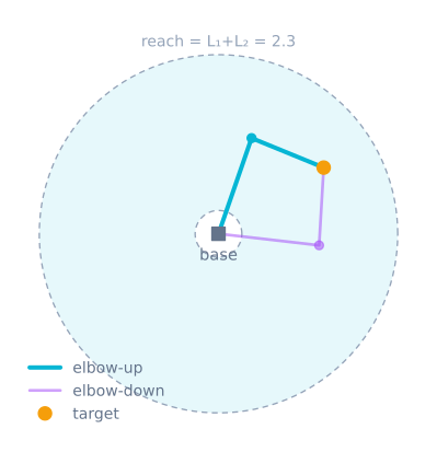
Near a singularity, a small tool motion can demand a very large joint motion. A planner must also respect position, velocity, acceleration, torque, and collision limits. Geometric reach alone does not make a trajectory safe.
Algorithm
- Define link lengths, joint axes, home transforms, and joint limits.
- Compute forward kinematics for the current joint state.
- Compare the current tool pose with the requested target.
- Use an analytic or numerical solver to reduce pose error within limits.
- Reject colliding or singular candidates and select a continuous solution.
- Time-parameterize the path and send synchronized setpoints to joint controllers.
Source code
A planar two-link arm has a compact forward model:
from math import cos, sin

def forward_kinematics(theta_1, theta_2, link_1, link_2):
    elbow = (link_1 * cos(theta_1), link_1 * sin(theta_1))
    tool = (
        elbow[0] + link_2 * cos(theta_1 + theta_2),
        elbow[1] + link_2 * sin(theta_1 + theta_2),
    )
    return elbow, tool
For physical arms, validate every planned trajectory in a bounded, collision-aware environment before enabling actuator power.
Assumptions and hardware differences
The arm is planar with two or three revolute joints, perfectly rigid links, instant velocity response and no gravity, dynamics or collision — you can swing from elbow-up to elbow-down with no torque limit. Real servos have position and velocity limits, gear backlash, current-limited torque and payload-dependent sag, and a 6-axis arm must also manage orientation, singularities and work near joint limits. This lab is where you learn why a target inside the annulus can have two solutions and why a target on its edge is singular, before you add the dynamics that make those poses hard to hold.
Circuit diagram
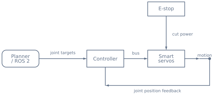
Separate high-current actuator power from compute power while maintaining the reference and safety signals required by the selected hardware.
Guided experiments
Dragging a target around is the fastest way to build intuition for things that are tedious to prove on paper and expensive to discover on hardware.
1. Find the shape of the workspace
Drag the target slowly outward until the solver reports unreachable, then trace that boundary all the way round. Now drag inward toward the base.
With unequal link lengths you will find two boundaries: an outer circle at L1 + L2 and an
inner one at |L1 − L2|. The workspace is an annulus, not a disc, and there is a hole in
the middle the arm physically cannot reach.
| Links | Outer reach | Inner hole | Shape |
|---|---|---|---|
| 100 + 90 | 190 | 10 | Annulus with a small hole |
| 100 + 50 | 150 | 50 | Annulus with a large hole |
| 100 + 100 | 200 | 0 | A full disc — equal links can fold onto themselves |
That last row is a genuinely useful design fact: equal link lengths remove the dead zone entirely. If your arm needs to work close to its own base, that is the reason to choose them.
2. Watch the two solutions merge
Toggle between the elbow-up and elbow-down branches at a target near the middle of the workspace: two clearly different arm poses reaching the same point.
Now drag that target outward toward the boundary. The two poses converge, and at full extension they become the same pose. That is a singularity, and it is where the arm loses the ability to move the tool in one direction no matter what the joints do.
3. Feel what a singularity costs
Drag the target along a straight line that passes near full extension, slowly and steadily. Watch the joint angles rather than the arm.
The tool moves at a constant rate; the joints do not. Near the boundary a small tool motion demands an enormous joint motion, so a smooth Cartesian path becomes a violent joint movement. On hardware that is a servo slamming to its limit.
Keep planned paths inside about 95% of maximum reach, and this stops being a problem.
4. Cross a branch boundary and watch the flip
Set the solver to always choose elbow-up, then drag the target through a region where that branch runs into a joint limit and the solver switches. The arm flips through a large, fast, completely unplanned motion.
This is why the right default is minimum motion — choose whichever branch is closest to the current pose — rather than a fixed branch. A silent mid-path branch switch on real hardware is alarming and can be destructive.
What you should observe
| Action | Expected result | If you see something else |
|---|---|---|
Target beyond L1 + L2 |
A clean “unreachable” | A NaN or a snapped pose means the solver is testing reachability too late |
Target inside |L1 − L2| |
Also unreachable | Correct — this is the hole, not a bug |
| Target behind the base | Reached correctly | If it mirrors, that is atan instead of atan2 |
| Toggle elbow branch | Same tool position, different joints | Both are valid; choosing is your decision |
| Drag toward the boundary | Joint rates rise sharply | This is the singularity |
| Round trip through FK then IK | The original angles come back | A mismatch means a sign or offset convention is inconsistent |
Taking it to hardware
The geometry transfers exactly. Nothing else does, and the gap is where a first arm build spends its time:
| This lab | A real servo arm |
|---|---|
| Joints go exactly where commanded | Servo zero is wherever the horn was fitted; some rotate the wrong way |
| No gravity | The shoulder sags at extension — worst exactly where accuracy is worst |
| No backlash | Several degrees of play, charged at every reversal |
| Instant motion | A commanded jump goes at full speed, with a current spike |
| Perfect link lengths | Measure between joint axes, not bracket edges |
| Infinite torque | An SG90 at 58% of stall will not hold position accurately |
Two numbers make the point. Four degrees of play at the shoulder over a 190 mm reach is more than 13 mm at the gripper — larger than any error the maths introduces. And a link length measured 10 mm long on a 95 mm link is a 10% systematic error that no tuning will remove.
The practical consequence is that hardware accuracy comes from calibration and consistent approach direction, not from better kinematics. Always approach a target from the same direction and the backlash becomes a repeatable offset you can subtract. The full solver, with every failure case handled, is in inverse kinematics for a two-link arm.
Hardware checklist
Components
- Three-axis or greater robot arm
- Controller capable of synchronized joint updates
- Joint feedback or smart servos
- Rigid base and defined tool center point
- Emergency stop and current-limited supply
Explore the graph
Where this simulator is used
The projects, learning paths, and tutorials that build on this lab.
Continue building
Download resources
Use these on-page references while working through the project. Downloadable project bundles will be added only after their source and version are published.
Common questions
Frequently asked questions
What is the difference between forward and inverse kinematics?
Forward kinematics calculates the tool pose from known joint values. Inverse kinematics starts with a desired tool pose and searches for one or more joint configurations that can produce it.
Why does a 2-link arm have two solutions (elbow-up and elbow-down)?
For most reachable targets the elbow can bend either way and still place the tool on the same point, giving an elbow-up and an elbow-down configuration. The two solutions come from the plus-or-minus in the law-of-cosines angle for the second joint. They coincide only at a singularity, where the arm is fully stretched or fully folded.
How do I choose between elbow-up and elbow-down?
Pick the configuration that is safest and most efficient for the task: one that keeps joints away from their limits, minimizes movement from the current pose, or avoids obstacles. This simulator lets you toggle between branches and shows the alternate solution as a ghost so the trade-off is visible.
What is a singularity in a robot arm?
A singularity is a configuration where the arm loses the ability to move the tool in some direction—typically when it is fully extended or fully folded. Near a singularity a small tool motion can demand a very large joint motion, so planners slow down or route around these poses. It is also where the elbow-up and elbow-down solutions merge into one.
When does inverse kinematics have no solution?
A planar two-link target is reachable only inside the annular ring between the shortest reach (the difference of the link lengths) and the longest reach (their sum). A point outside that ring cannot be reached at any joint angle. A pose can also be unreachable because it needs a forbidden joint angle, an orientation the available joints cannot achieve, or would collide with the arm itself.
Why use analytic inverse kinematics instead of a numerical solver?
For a two- or three-link planar arm the geometry has a closed-form (analytic) solution, so you can compute the exact joint angles directly, deterministically, and fast—ideal for teaching and testing. Numerical solvers are needed for redundant or spatial arms where no closed form exists, but they iterate, can miss solutions, and are harder to reason about.
Further reading
References
Authoritative sources for going deeper than this simulator's bounded educational model.