
PID Controller Simulator for Robotics Control Systems
Tune proportional, integral, and derivative gains while visualizing response, error, saturation, and disturbances in a PID controller simulator.
- Category
- Control Systems
- Time
- 60–120 min
- Platform
- Browser · Arduino
01 / Start here
Introduction
PID control appears throughout robotics: wheel speed, heading, joint position, temperature, and balancing systems all rely on feedback. This project turns the controller into a visible experiment. Change one gain, disturb the plant, and connect the resulting curve with the code that could run on an Arduino or embedded controller.
Live lab / Deterministic sampled control loop
PID controller simulator
Drive a second-order plant toward a setpoint. Tune each gain, inject a load, and watch response, error, and control effort in real time.
Three stacked plots share a scrolling time axis: measured output against the setpoint line, tracking error around zero, and control effort inside the shaded actuator-limit band.
- Setpoint
- 1.00
- Measured
- 0.000
- Error
- 1.000
- Control
- 0.000
- Overshoot
- 0%
- Steady-state error
- 1.000
Keyboard: focus the plots, then use Space to run/pause, N to step, R to reset, G to toggle the load, and F for full screen.
Controls
The simulator exposes setpoint, proportional, integral, and derivative gains, sample interval, actuator limit, and disturbance magnitude. Aligned plots show setpoint, measured output, error, and control effort. Reset clears controller memory so experiments remain comparable.
Theory
A feedback controller calculates error as setpoint minus measurement. Proportional action reacts immediately, integral action accumulates persistent error, and derivative action responds to the rate of change. Their sum becomes the actuator command.
Controller performance is constrained by the plant. Sampling too slowly hides motion; driving beyond the actuator limit causes saturation; noisy measurements make an unfiltered derivative term unstable. Tuning is therefore an experiment involving both controller and system.
Algorithm
- Read the measurement at a fixed interval and compute error.
- Accumulate a bounded integral using the actual time step.
- Estimate derivative from measurement or error and apply appropriate filtering.
- Sum the three weighted terms and clamp to the actuator range.
- Apply the command, store the previous sample, and record metrics.
- Reset integral and history when the control mode or plant changes substantially.
Source code
This implementation includes a simple anti-windup condition:
float updatePid(float setpoint, float measured, float dt) {
  const float error = setpoint - measured;
  const float derivative = (error - previousError) / dt;
  const float candidateIntegral = integral + error * dt;
  const float raw = kp * error + ki * candidateIntegral + kd * derivative;

  const float output = constrain(raw, outputMin, outputMax);
  if (raw == output) integral = candidateIntegral;
  previousError = error;
  return output;
}
Production controllers also define behavior for invalid measurements, timer overruns, mode transitions, and actuator faults.
Assumptions and hardware differences
The plant here is a clean second-order model with known mass, damping and delay that you set with the sliders — not a real motor with friction, deadband, torque that fades with speed, and a driver that heats up. Sampling is fixed by construction, so the derivative term stays well-behaved; on an Arduino, delay() or other blocking work makes the interval jitter and the D term misbehave even when the gains are unchanged. Actuator saturation is modelled as a hard clamp with anti-windup provided, but a physical system also has current limits, supply sag and heat that change the limit while running. Tune the shape here, then verify on hardware where the plant is only approximately known.
Circuit diagram
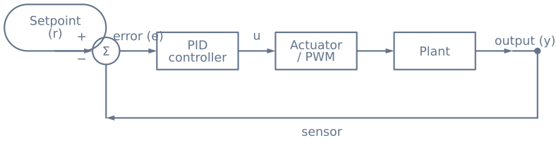
The feedback sensor reports the actual output; it is not a substitute for current limiting or a hardware safety stop. The controller compares the setpoint with the conditioned sensor reading, then drives the actuator through a PWM stage rated for the load.
Guided experiments
Reading about overshoot is not the same as producing it deliberately. Each experiment below takes a couple of minutes and isolates exactly one effect.
1. Find the ultimate gain
Set Ki and Kd to zero. Raise Kp until the output oscillates at a constant amplitude —
neither growing nor decaying. Note that gain (Ku) and the oscillation period (Tu).
Those two numbers are all you need for a first tune:
| Controller | Kp |
Ki |
Kd |
|---|---|---|---|
| PID (classic) | 0.6 Ku |
1.2 Ku / Tu |
0.075 Ku Tu |
| PID (no overshoot) | 0.2 Ku |
0.4 Ku / Tu |
0.066 Ku Tu |
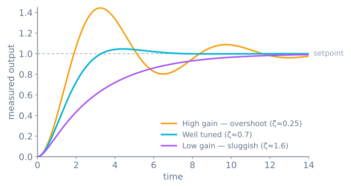
Type those in and compare. The classic row is aggressive and overshoots 20–40%; the second lands without overshoot and takes longer. Neither is “correct” — they are different answers to different requirements, which is the point.
2. Watch integral windup happen
Set the actuator limit low — around 20% of its range — then command a large setpoint step. Watch the control-effort plot: it saturates immediately and stays there, while the integral keeps accumulating error it cannot act on. When the output finally reaches the setpoint, all that stored action unwinds and the system sails far past.
Now raise the actuator limit and repeat with the same gains. The overshoot largely disappears. Nothing about the controller changed — which is the lesson. Windup is a property of the interaction between the controller and a saturating actuator, not of the gains.
3. Prove that lag, not noise, is what kills a loop
Raise the sample interval from its lowest value in steps, keeping the gains fixed. The response degrades long before the plot looks noisy: overshoot grows, then oscillation appears, then it goes unstable.
| Sample interval | What you see with an otherwise good tune |
|---|---|
| 5 ms | Clean, as tuned |
| 20 ms | Slightly more overshoot |
| 50 ms | Visible ringing |
| 100 ms | Sustained oscillation |
| 200 ms | Unstable |
This is why removing a delay() from a robot’s loop often improves tracking more than any
amount of tuning. Stale information cannot be recovered by a gain.
4. Feed the derivative some noise
Raise the disturbance magnitude with Kd at zero, then raise Kd. The control-effort trace
becomes jagged well before the output does — you are watching differentiation amplify
high-frequency content, exactly as it must.
That behaviour is why people conclude D is useless and set it to zero. The real fix is upstream: filter the measurement, or filter the derivative term itself.
What you should observe
| Setting | Expected shape | If you see something else |
|---|---|---|
Kp alone, low |
Rises slowly, settles below the setpoint | — |
Kp alone, high |
Overshoots, rings, decays | Growing oscillation means you are past Ku |
Kp + Kd |
Fast rise, little overshoot, small steady offset | Jagged effort means D is amplifying noise |
Kp + Ki |
Reaches the setpoint exactly, slower | Sails past means windup or too much Ki |
| Full PID | Fast, minimal overshoot, no offset | — |
The steady offset with P and D but no I is worth producing deliberately once. It is the clearest demonstration of what the integral term is actually for: proportional action needs a non-zero error to produce any output at all, so it necessarily parks slightly short.
Taking it to hardware
Gains found here are a starting point, not a transfer. What transfers perfectly is the procedure; what does not transfer is the numbers, because they describe this plant.
| This lab | A real robot |
|---|---|
| Sample interval is exact | Jitters unless you measure dt and pass it in |
| The plant is a clean second-order model | Friction, deadband, torque that fades with speed |
| Actuator limit is a hard clamp | Also current limits, supply sag, and heat |
| No sensor noise unless you add it | Always noise, and rarely Gaussian |
| The plant never changes | Battery voltage, load and temperature all change it |
The last row causes the most confusion in practice. A tune that is perfect on fresh cells will be sluggish on flat ones, because the same command now produces less torque. That is not a failure of the method — gains are properties of the plant, and the plant moved. The professional answers are a speed loop underneath, or gain scheduling. Work through how to tune a PID controller for the full procedure, then bring it to the line follower lab where the plant fights back.
Hardware checklist
Components
- Microcontroller with a stable timer
- Measured plant such as a DC motor or servo
- Encoder, potentiometer, or other feedback sensor
- Output driver rated for the actuator
- Regulated power source and emergency stop
Explore the graph
Where this simulator is used
The projects, learning paths, and tutorials that build on this lab.
Continue building
Download resources
Use these on-page references while working through the project. Downloadable project bundles will be added only after their source and version are published.
Common questions
Frequently asked questions
What should I tune first?
Begin with integral and derivative gains at zero. Increase proportional gain until the response is useful but oscillatory, then add derivative damping. Add integral gain last and only when a repeatable steady-state error remains. A common rule of thumb: P gives speed, D reduces overshoot, and I removes offset—add them in that order, one at a time.
How do I stop a PID controller from overshooting?
Overshoot usually comes from too much proportional or integral action. Reduce proportional gain first, then increase derivative gain to damp the approach. If overshoot only appears after the actuator hits its limit, the cause is integral windup rather than gain, and you should clamp the integral term instead.
Why does my PID controller oscillate?
Sustained oscillation almost always means the proportional gain is too high for the loop, or the derivative term is too weak to damp it. Reduce proportional gain by about half, then add derivative gain. Oscillation can also come from a control loop that runs too slowly or with an inconsistent interval, which makes the derivative term unreliable.
What is integral windup and how do I prevent it?
Windup occurs when the actuator saturates—a motor at full speed, a valve fully open—but the accumulated integral error keeps growing, so the controller overshoots badly when the error finally reverses. Prevent it with clamping (stop adding to the integral while the output is saturated) or back-calculation (bleed the integral down using the difference between the requested and delivered output).
How fast does a PID loop need to run?
The loop should sample several times faster than the system it controls, at a consistent interval. On a microcontroller, avoid long blocking delays: a variable or slow loop changes the effective integral and derivative terms even when the gains are unchanged, which is a frequent hidden cause of poor tuning.
Can I use PID with only the P and D terms?
Yes. PD control (no integral) is common when a small steady-state error is acceptable and you want to avoid windup, and PI control (no derivative) suits noisy signals where a derivative term would amplify noise. Use only the terms the problem needs rather than always running full PID.
What is the difference between manual tuning and Ziegler–Nichols?
Manual tuning adjusts one gain at a time while watching the response, which is intuitive and safe for learning. Ziegler–Nichols is a formula-based method that derives gains from the point of sustained oscillation; it is faster but often aggressive, so its output is usually a starting point you refine by hand.
Further reading
References
Authoritative sources for going deeper than this simulator's bounded educational model.