
Obstacle Avoidance Simulator for Mobile Robots
Learn reactive navigation, range sensing, and safe stopping with an obstacle avoidance robotics simulator for Raspberry Pi projects.
- Category
- Raspberry Pi
- Time
- 2–3 hours
- Platform
- Browser · Raspberry Pi
01 / Start here
Introduction
Obstacle avoidance turns incomplete, noisy measurements into safe motion. This project separates perception, safety, and steering so you can reason about each layer before deploying a mobile robot. The simulator exposes sensor coverage, stopping distance, and failure cases rather than pretending a single reactive rule solves every navigation problem.
Live lab / Reactive range-sensing navigation
Obstacle avoidance simulator
Drive a mobile robot toward the goal while a fan of range sensors keeps it clear of obstacles. Reposition the scene by dragging or with the coordinate controls, add noise, and compare two steering rules.
Lines are sensor rays; a brighter ray marks the nearest reading. The dashed line ahead is the predicted stopping distance. The green ring is the goal. Drag a scene item or use the position controls below.
- Status
- Seeking
- Distance to goal
- 630 px
- Min clearance
- 170 px
- Stopping distance
- 24 px
- Elapsed
- 0.0 s
Keyboard: focus the workspace, then use Space to run/pause, N to step, R to reset, D to add an obstacle, and F for full screen.
Controls
The workspace includes movable obstacles, robot speed, sensing range, field of view, measurement noise, and a safety-distance threshold. Sensor rays and predicted stopping distance stay visible. Step mode reveals exactly which observation caused each steering decision.
Theory
A robot must stop or turn before its swept footprint intersects an obstacle. Safe distance depends on current velocity, controller latency, braking capability, measurement uncertainty, and the robot’s physical radius—not just the latest range value.
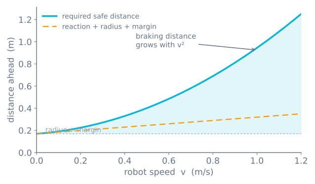
Reactive controllers such as potential fields turn nearby obstacles into repulsive vectors and the goal into an attractive vector. They respond quickly but can become trapped in local minima. A practical stack pairs reactive safety with a global or local planner.
Algorithm
- Reject stale and physically impossible range samples.
- Transform valid observations into the robot coordinate frame.
- Expand each obstacle by the robot radius plus a safety margin.
- Compute stopping distance from velocity and estimated deceleration.
- Stop when the forward corridor is unsafe; otherwise steer toward the clearest goal-aligned sector.
- Limit acceleration and angular velocity before sending motor commands.
Source code
Keep the emergency decision small enough to test exhaustively:
def safe_velocity(target, ranges, stop_distance):
    front = [r for angle, r in ranges if abs(angle) < 0.35]
    if not front or min(front) <= stop_distance:
        return 0.0, choose_clear_turn(ranges)
    return limit_acceleration(target), steer_toward_clearance(ranges)
In a real system, record sensor timestamps and enter a safe stopped state when required data becomes unavailable.
Assumptions and hardware differences
The world is top-down and two-dimensional: sensor rays are instant, perfectly thin, and never occluded by the robot’s own body, and the robot is a disk that can brake to zero without momentum. On a Raspberry Pi robot, ultrasonic beams spread 15°, time-of-flight readings depend on surface and sun, and stopping distance is set by real mass, motor torque and sense-decide-actuate latency — all covered in the reactive navigation roadmap. The simulator also ignores loop jitter and power sag, so treat the stopping-distance curve as the shape to internalise, not a number to copy.
Circuit diagram
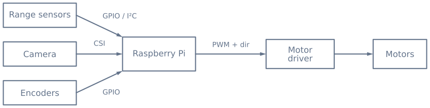
Level-shift any 5 V echo signal before it reaches Raspberry Pi GPIO. Power motors separately and connect grounds at a deliberate common point.
Guided experiments
1. Derive the stop threshold instead of guessing it
Set a low speed and lower the stop threshold until the robot starts clipping obstacles. Note the value. Now double the speed and repeat.
The threshold you need does not double, because it is the sum of a term that scales with speed and one that scales with its square:
stop_distance = (v x t_latency) + (v^2 / (2 x a_brake)) + robot_radius + margin| Speed | Latency term (80 ms) | Braking term (1 m/s²) | Total, with 90 mm radius + 50 mm margin |
|---|---|---|---|
| 0.15 m/s | 12 mm | 11 mm | 16 cm |
| 0.30 m/s | 24 mm | 45 mm | 21 cm |
| 0.60 m/s | 48 mm | 180 mm | 37 cm |
| 0.90 m/s | 72 mm | 405 mm | 62 cm |
This is why a robot that avoids reliably at walking pace starts hitting things when you speed it up — and why the fix is a speed-dependent threshold rather than one large fixed value that makes the robot timid everywhere.
2. Produce the threshold stutter, then fix it
Park the robot so it hovers right at the stop distance. With a single threshold it flips between driving and turning many times a second.
Now separate the two: stop at 20 cm, and do not resume until 30 cm. The stutter disappears because the behaviour has to commit. That gap is hysteresis, and the same pattern fixes almost every threshold-driven oscillation in robot code.
3. Trap it deliberately
Build a concave corner — a horseshoe — and let the robot drive in. With a deterministic “turn toward the most open direction” rule it will turn, drive, and arrive back where it started, forever.
This is not a bug to fix. It is what having no map means, and it is the clearest possible demonstration of the ceiling of reactive navigation. The mitigations are a random component in the turn and a stuck-detector that escalates after several failed attempts; the actual fix is memory, which is a different path entirely.
4. Compare scan resolution against scan time
Increase the number of scan angles and watch two things move in opposite directions: the turn decisions get better, and the robot spends longer standing still.
A scan is a blind moment — the robot is stopped and making no progress. Three to five angles is the usual sweet spot, and past that the extra information rarely justifies the extra time.
What you should observe
| Behaviour | Cause |
|---|---|
| Clips obstacles at speed | Threshold not scaled for the quadratic braking term |
| Stutters at a fixed distance | One threshold, no hysteresis |
| Dithers left-right on the spot | Re-deciding before the turn has changed anything |
| Loops forever in a corner | Deterministic escape from a symmetric trap |
| Stops far too early everywhere | Threshold set for the worst case rather than the current speed |
| Turns toward the edge of a gap | Picking the maximum angle rather than a weighted centroid |
Taking it to hardware
The simulator’s rays are instant, noise-free, and infinitely thin. A real ultrasonic sensor is none of those, and the differences are the whole of the work on hardware:
| This lab | An HC-SR04 on a real robot |
|---|---|
| A thin ray | A ~15° cone, about 53 cm across at 1 m |
| Every surface reflects | Soft and steeply angled surfaces return nothing at all |
| Instant readings | Up to 25 ms per ping, ~60 ms between them |
| No servo | 100–200 ms of settle time per scan angle |
| No noise | Occasional wild values needing a median filter |
| Sees everything | A curtain is invisible — which is why you fit bump switches |
Find a safe stopping distance and a clear-direction rule here, where a mistake costs nothing. Then on hardware, add the median filter, the servo settle delay, and the contact sensing — the avoidance algorithm tutorial has each in code.
Hardware checklist
Components
- Raspberry Pi with a supported power supply
- Two or more time-of-flight or ultrasonic sensors
- Optional camera module for visual detection
- Motor driver with separate motor supply
- Differential-drive chassis and encoders
Explore the graph
Where this simulator is used
The projects, learning paths, and tutorials that build on this lab.
Continue building
Download resources
Use these on-page references while working through the project. Downloadable project bundles will be added only after their source and version are published.
Common questions
Frequently asked questions
Why is one front-facing sensor not enough?
A single beam leaves blind areas near the robot and cannot distinguish a narrow object from a wall. Multiple viewpoints or a scanning sensor provide enough geometry to choose a safer turn.
Does obstacle avoidance replace path planning?
No. Reactive avoidance handles immediate hazards, while a planner selects progress toward a goal. Robust robots combine both and let the safety layer override unsafe planned motion.
Ultrasonic or time-of-flight sensor — which is better for obstacle avoidance?
Ultrasonic sensors are cheap and work on most surfaces but have poor angular resolution and a blind zone close to the sensor. Time-of-flight (ToF) sensors give faster, more precise short-range distance and a narrow beam, but can be disturbed by strong sunlight, dark or mirror-like surfaces, and corner reflections. Many robots use ultrasonic for coarse coverage and ToF where precise short-range sensing matters.
What is a sensor blind zone and why does it matter?
The blind zone is the minimum range below which a sensor cannot report a valid distance—for ultrasonic sensors it is set by the length of the emitted pulse. An obstacle inside the blind zone reads as clear, so a robot that trusts the raw value can drive into something right in front of it. Keep sensors mounted so the blind zone falls inside the robot's own footprint, and treat suspiciously small readings as invalid.
How do I calculate a safe stopping distance?
Safe distance is reaction distance plus braking distance plus the robot's radius and a margin. Reaction distance grows linearly with speed (speed times sense-decide-actuate latency), but braking distance grows with the square of speed, so required clearance rises faster than speed itself. This is why a small speed increase can demand a much larger safe gap.
Why does my robot get stuck in front of an obstacle?
Reactive methods such as potential fields can reach a local minimum where the repulsive push from an obstacle cancels the attraction to the goal, and the robot stalls or oscillates. Follow-the-gap steering that commits to the widest clear opening, plus a global or local planner above the reactive layer, keeps the robot from trapping itself.
How do I filter noisy distance readings?
Reject physically impossible values and sudden jumps rather than acting on them, timestamp every sample, and apply a light median or temporal filter to suppress spurious echoes. If required data goes stale or unavailable, enter a safe stopped state instead of steering on a guess.
Further reading
References
Authoritative sources for going deeper than this simulator's bounded educational model.