
Robot Sensor Simulator for Calibration and Sensor Fusion
Explore noise, bias, drift, quantization, dropouts, filtering, and fusion in a deterministic interactive robot sensor simulator.
- Category
- Sensors
- Time
- 60–150 min
- Platform
- Browser · Microcontroller
01 / Start here
Introduction
Robots act on measurements that are delayed, biased, noisy, and incomplete. This project makes those limitations visible. Compare truth, raw samples, and filtered estimates; change sampling conditions; and learn how calibration affects downstream control without mistaking an educational model for a specific sensor.
Live lab / Deterministic measurement model
Robot sensor simulator
Compare a known signal with noisy absolute readings and a filtered estimate. Change one error source at a time to see what calibration can—and cannot—fix.
The main plot compares solid truth, individual absolute-sensor samples, and the thicker dashed estimate. The lower band shows signed estimation error around zero; gaps mark dropped absolute samples.
- Truth
- —
- Absolute
- —
- Estimate
- —
- Error
- —
- RMSE
- —
- Dropped
- 0
Keyboard: focus the plot, then use Space to run/pause, N to step, R to reset, and F for full screen.
Controls
Choose a smooth or stepped truth signal, then adjust sample rate, quantization, random noise, drift, bias, dropouts, and filter memory. Compare raw data with moving-average, low-pass, median, and complementary estimates. Presets make noisy, biased, and unreliable sensor behavior repeatable.
Theory
Every sensor has a measurement range, resolution, accuracy, bandwidth, latency, and failure behavior. Datasheet accuracy describes only part of the system; mounting, temperature, supply noise, electromagnetic interference, and surface properties often dominate real results.
Fusion works when sensors contribute complementary information and their uncertainty is represented honestly. Combining two biased measurements does not automatically create truth. Start with calibration, timestamps, coordinate frames, and data-quality checks.
Algorithm
- Timestamp and range-check every sample at the acquisition boundary.
- Convert raw units using calibration scale, offset, and axis alignment.
- Reject impossible jumps or mark them invalid instead of inventing data.
- Apply the lightest filter that meets the downstream noise requirement.
- Transform measurements into a common frame and fuse them using known uncertainty.
- Log raw and processed values so failures remain reproducible.
Source code
An exponential low-pass filter is useful when its time constant is chosen deliberately:
class LowPass:
    def __init__(self, alpha):
        self.alpha = alpha
        self.value = None

    def update(self, sample):
        if self.value is None:
            self.value = sample
        else:
            self.value += self.alpha * (sample - self.value)
        return self.value
Record the raw sample beside the filtered result. Otherwise an attractive plot can hide clipping, dropouts, and calibration errors.
Assumptions and hardware differences
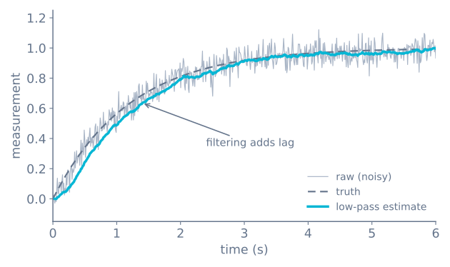
This lab is an educational signal model, not a specific sensor datasheet. Noise is seeded Gaussian or uniform with a dial you control; a real IMU or ToF sensor adds temperature-dependent bias, non-Gaussian spikes and bus timing jitter that this model simplifies. Sampling is perfectly periodic here, but on a microcontroller loop timing and interrupt latency make timestamps essential — which is why every processing mode in the controls compares truth, raw samples and the estimate together. Filtering looks attractive on a plot, yet every smoother adds lag that will later appear as control delay on hardware; the same trade is covered in the sensor noise tutorial.
Circuit diagram
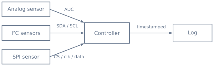
Confirm bus voltage, pull-up requirements, addresses, and maximum cable length before connecting multiple sensors.
Guided experiments
The dials in this lab exist to let you produce each sensor fault deliberately, then see which tool fixes it. Doing that once is worth a great deal of reading.
1. Prove that filtering cannot fix a bias
Set noise to zero and bias to a clear offset. Now try every filter in turn — moving average, low-pass, median. None of them move the estimate toward the truth, because all three attenuate variation and a bias does not vary.
Then set bias to zero and noise high, and watch the same filters work well. This is the single most useful distinction in sensor work: noise, bias and drift look alike on a plot and need three different fixes, and more filtering never cures a bias.
2. Watch a mean smear a spike that a median rejects
Turn on dropouts or spikes, and compare a moving average against a median of the same window.
| Filter | What one outlier does |
|---|---|
| Moving average of 5 | Shifts the estimate for five consecutive samples |
| Median of 5 | Contributes nothing at all |
Ultrasonic and time-of-flight noise is not Gaussian — it is occasional wild values against an otherwise steady signal. That is exactly the case an average handles worst.
3. Measure what the lag costs you
Switch to the stepped truth signal and lower the filter’s alpha (or lengthen the window). The
estimate gets smoother and arrives later. Read the delay off the plot at each setting:
| Filter setting | Typical lag | At 0.3 m/s that is |
|---|---|---|
| Median of 3 | ~1 sample | 3 mm |
| Moving average of 10 | ~4.5 samples | 14 mm |
| Low-pass, α = 0.1 | ~9 samples | 27 mm |
| Low-pass, α = 0.02 | ~49 samples | 147 mm |
The last row produces a beautifully smooth trace and steers a robot on where the obstacle was 15 cm ago. Always check the lag in the units the robot cares about, not in samples — this is the most common way a well-intentioned filter makes a robot worse.
4. See what fusion can and cannot do
Set one source noisy-but-unbiased and the other smooth-but-drifting, and watch the complementary estimate take the good half of each. Then give both sources the same bias and watch the fused estimate inherit it exactly.
Fusion exploits errors that are independent. A common-mode error survives untouched, which is why calibration comes before fusion rather than after it.
What you should observe
| Configuration | Raw | Best filter | Why |
|---|---|---|---|
| Gaussian noise, no bias | Scatters symmetrically | Moving average or low-pass | Noise averages toward truth |
| Occasional spikes | Mostly good, rare wild values | Median | Rejects outliers outright |
| Constant offset | Tight but wrong | None — calibrate | Filtering cannot see the offset |
| Slow drift | Starts right, walks away | None — recalibrate or fuse | Needs an absolute reference |
| Dropouts | Gaps | Median, plus hold-last-good | An invented value is worse than a marked gap |
| Quantised | Lands on discrete steps | None — this is your resolution | Filtering between steps adds lag, not information |
Taking it to hardware
| This lab | A real sensor |
|---|---|
| Sampling is perfectly periodic | Loop timing and interrupt latency make timestamps essential |
| Noise is seeded Gaussian or uniform | Non-Gaussian spikes, and bias that moves with temperature |
| Truth is available for comparison | You have no truth — which is why you calibrate against a known input |
| Dropouts are explicit | A dropout can look like a plausible value |
| One sensor at a time | Several buses, several rates, and alignment problems between them |
The practical procedure for a real sensor is short: hold it still against a known input, log a few thousand timestamped samples, and plot both the time series and a histogram. The histogram is the part people skip and the most informative — Gaussian noise makes a bell, outliers make a bell with a few points far out in the tails, and those two need different filters. The full method is in sensor noise, bias, and filtering.
Hardware checklist
Components
- Microcontroller or single-board computer
- One or more digital or analog sensors
- Known calibration references
- Stable regulated supply and correct logic levels
- Logging connection for repeatable experiments
Explore the graph
Where this simulator is used
The projects, learning paths, and tutorials that build on this lab.
Continue building
Download resources
Use these on-page references while working through the project. Downloadable project bundles will be added only after their source and version are published.
Common questions
Frequently asked questions
Is a smoother signal always a better signal?
No. Strong filtering can remove useful motion and introduce delay. Choose a filter from the noise spectrum, required response time, and the decisions that consume the measurement.
What is the difference between bias and noise?
Bias is a repeatable offset from the true value, while noise varies between samples. Calibration can estimate bias; averaging or filtering may reduce random noise but cannot reliably remove an unknown bias.
What is sensor drift, and how is it different from bias?
Bias is a fixed offset you can measure once and subtract. Drift is a slow change in that offset over time, usually with temperature or component aging, so a calibration taken at startup gradually stops matching reality. Drift is why long runs need periodic recalibration or a reference the estimator can correct against.
Which filter should I use: moving average, low-pass, or median?
A moving average and an exponential low-pass both smooth Gaussian-style noise, trading responsiveness for smoothness through their window or time constant. A median filter is better at removing occasional spikes and dropouts because a few bad samples do not move the middle value. Pick the lightest filter that meets the downstream requirement rather than the smoothest-looking one.
How much delay does filtering add?
Every smoothing filter lags the true signal, and more smoothing means more lag: a low-pass filter with a long time constant rejects more noise but falls further behind fast changes. Always plot the filtered estimate against the raw samples and the truth so the lag is visible before you rely on it in a control loop.
What is sensor fusion and when does it actually help?
Fusion combines multiple sensors into one estimate, and it helps only when the sensors contribute complementary information and their uncertainty is represented honestly. Combining two biased measurements does not create truth. A complementary filter, for example, trusts one sensor at high frequencies and another at low frequencies; start with calibration, timestamps, and coordinate frames before fusing.
Why should every sample be timestamped?
Samples rarely arrive at a perfectly fixed interval, and fusion and filtering assume you know when each value was measured. Timestamps let you detect jitter, align data from different sensors, and reject stale readings. Logging raw values beside processed ones keeps failures such as clipping, dropouts, and calibration errors reproducible.
Further reading
References
Authoritative sources for going deeper than this simulator's bounded educational model.