
Tutorial · Beginner · 18 min read
How to Tune a PID Controller: A Practical Guide
Tune a PID controller step by step: set proportional gain first, add derivative to stop overshoot, add integral last, and avoid integral windup.
A PID controller turns the error between where a system is and where you want it to be into a correction. It has three terms—proportional, integral, and derivative—and tuning is the process of choosing how strongly each one acts. The reliable way to do it is one term at a time, in a fixed order, watching the response after every change. You can follow along in the PID Controller Simulator.
Start with proportional gain
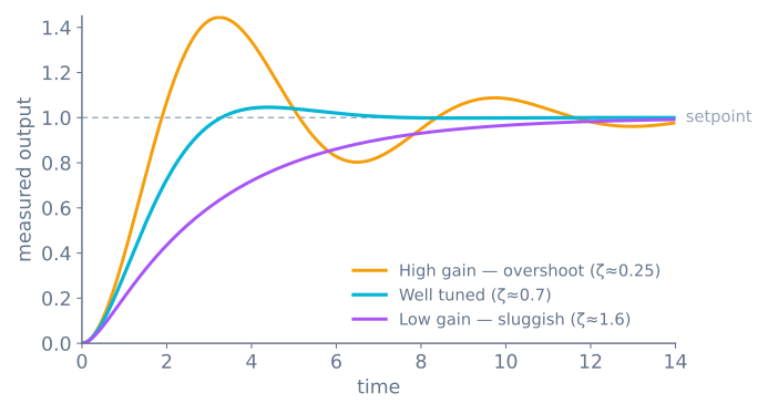
Set the integral and derivative gains to zero. Raise the proportional gain (Kp) until the system responds quickly to a change in setpoint. Too little and it reacts sluggishly; too much and it overshoots and oscillates. Stop when the response is fast but only lightly oscillatory—this is your working point for adding the other terms.
A useful rule: P gives you speed. It reacts to the error right now, and nothing else.
Add derivative to tame overshoot
Now raise the derivative gain (Kd). Derivative action responds to how fast the error is changing, so it applies the brakes as the system approaches the setpoint. This is what removes the overshoot and ringing that pure proportional control leaves behind.
Add just enough derivative to settle the oscillation. Too much makes the controller twitchy, because the derivative term amplifies any noise in the measurement. If your signal is noisy, filter it before differentiating, or lean on proportional and integral instead.
Add integral last
Proportional and derivative together can still leave a small, steady offset—the system parks just short of the setpoint. The integral term (Ki) fixes that: it accumulates error over time and pushes until the offset is gone.
Add integral gain slowly and only if a repeatable steady-state error remains. Integral is the slowest term and the easiest to overdo, so a little goes a long way.
Watch for integral windup
Integral windup is the classic PID failure. When the actuator saturates—a motor already at full speed, a valve fully open—the system cannot respond, but the integral term keeps accumulating error. When the error finally reverses, all that stored-up action unwinds at once and the system overshoots badly.
Prevent it by clamping the integral (stop adding to it while the output is saturated) or by back-calculation (bleed the integral down using the gap between the requested and delivered output). A simple clamp:
float candidateIntegral = integral + error * dt;
float raw = kp * error + ki * candidateIntegral + kd * derivative;
float output = constrain(raw, outputMin, outputMax);
if (raw == output) integral = candidateIntegral; // only accumulate when not saturated
Keep the loop timing honest
All three terms depend on a consistent time step. On a microcontroller, a long delay() in the loop adds dead time that makes the derivative term useless no matter how high you set it, and it distorts the integral. Run the loop fast and at a steady interval, and pass the real elapsed time into the calculation.
Getting close fast: the Ziegler–Nichols starting point
Raising P until you find the oscillation is not just a sanity check — it gives you a number you can compute the whole tune from. Set I and D to zero, raise P until the output oscillates steadily without growing or decaying, and record two things:
Ku— the proportional gain at which that happens (the ultimate gain)Tu— the period of the oscillation, in seconds
Then:
| Controller | Kp |
Ki |
Kd |
|---|---|---|---|
| P only | 0.5 Ku |
— | — |
| PI | 0.45 Ku |
0.54 Ku / Tu |
— |
| PID (classic) | 0.6 Ku |
1.2 Ku / Tu |
0.075 Ku Tu |
| PID (no overshoot) | 0.2 Ku |
0.4 Ku / Tu |
0.066 Ku Tu |
These are a starting point, not an answer. The classic row is deliberately aggressive and typically overshoots 20–40%, which is fine for a motor and unacceptable for a robot arm near a table. The last row trades response speed for landing without overshoot.
The value of the method is that it replaces three unknowns with two measurements. Twenty
minutes finding Ku and Tu gets you closer than an afternoon of guessing, and you can then
tune by feel from a sensible place.
Take the derivative of the measurement, not the error
This is a one-line change that fixes the single most common complaint about D.
When the setpoint steps, the error steps with it. The derivative of a step is briefly enormous, so the controller commands a violent correction for a reason that has nothing to do with physics — nothing moved, you just asked for something different. On a robot this is a hard jerk every time you change the target.
// Derivative kick: the setpoint step goes straight into the output.
float derivative = (error - lastError) / dt;

// Derivative on measurement: the setpoint contributes nothing at all.
float derivative = -(measurement - lastMeasurement) / dt;
The sign flips because error is setpoint − measurement, so differentiating the measurement
instead means negating. When the setpoint is constant the two forms are mathematically
identical; when it changes, only the second behaves.
Use derivative on measurement unless you have a specific reason not to. There is almost no case where the kick is wanted.
Filter the derivative, or D will amplify your noise
Differentiation amplifies high-frequency content, and sensor noise is high-frequency by definition. A signal with ±2 counts of jitter sampled every 10 ms produces a derivative estimate swinging by ±200 counts per second — which D then turns into motor commands.
The usual result is that people conclude D is useless and set it to zero. The real problem is upstream:
// A first-order filter on the derivative term only.
// alpha = dt / (tau + dt); tau is the filter time constant in seconds.
const float tau = 0.05f;                       // 50 ms
const float alpha = dt / (tau + dt);
dFiltered += alpha * (dRaw - dFiltered);
Choosing tau is a trade: too small and the noise survives, too large and D is acting on
information that is already stale, which is exactly what D exists to avoid. Start at three
to five times your loop period and increase only until the twitching stops.
A complete controller
Everything above, in one place:
struct Pid {
  float kp, ki, kd;
  float outMin, outMax;
  float tau;                 // derivative filter time constant

  float integral = 0;
  float lastMeasurement = 0;
  float dFiltered = 0;
  bool  primed = false;
};

float pidUpdate(Pid &c, float setpoint, float measurement, float dt) {
  if (dt <= 0) return 0;

  const float error = setpoint - measurement;

  // Derivative on measurement, low-pass filtered.
  if (!c.primed) { c.lastMeasurement = measurement; c.primed = true; }
  const float dRaw = -(measurement - c.lastMeasurement) / dt;
  const float alpha = dt / (c.tau + dt);
  c.dFiltered += alpha * (dRaw - c.dFiltered);
  c.lastMeasurement = measurement;

  // Provisional integral, committed only if the output does not saturate.
  const float candidate = c.integral + error * dt;
  const float raw = c.kp * error + c.ki * candidate + c.kd * c.dFiltered;
  const float out = constrain(raw, c.outMin, c.outMax);
  if (raw == out) c.integral = candidate;      // conditional integration

  return out;
}
Three things in there are the difference between a controller that works on a robot and one that works in a textbook: derivative on measurement, a filtered derivative, and conditional integration so the integral cannot wind up while the actuator is saturated.
Diagnosing from the shape of the response
You can name almost every tuning fault from the response curve alone:
| What you see | What it means | What to change |
|---|---|---|
| Rises slowly, never arrives | P too low, no I | Raise P; add I if an offset remains |
| Settles short of the target, permanently | No integral term | Add I, slowly |
| Overshoots once, then settles | Slightly high P, no D | Add D |
| Overshoots repeatedly, decaying | P too high | Lower P, or add D |
| Oscillates forever at constant amplitude | P at the ultimate gain | You have found Ku — halve it |
| Oscillation grows | P above Ku |
Reduce immediately |
| Fast, jagged, jittery output | D acting on noise | Filter the derivative, or filter the sensor |
| Jerks hard whenever the setpoint changes | Derivative kick | Derivative on measurement |
| Sails far past after a big move | Integral windup | Conditional integration or a clamp |
| Was fine yesterday, sluggish today | Plant changed — usually the battery | Gains are properties of the plant, not the code |
That last row deserves emphasis because it is not a bug. Gains describe a specific plant, and the plant includes battery charge, chassis mass, surface, and gearbox temperature. A tune that was perfect on fresh cells will be sluggish on flat ones, because the same duty cycle now produces less torque. The professional answers are a speed loop underneath (so the controller commands speed, not duty) or gain scheduling (several tunes, selected by operating condition).
Loop timing, quantified
Both I and D are computed against elapsed time, so a loop that runs whenever it happens to finish computes both against a lie.
| Loop behaviour | Effect on the controller |
|---|---|
| Fixed interval | Everything works as designed |
Variable, but dt measured and passed in |
Also correct — this is the practical answer |
Variable, dt assumed constant |
I accumulates wrongly; D is noise |
Contains a delay() |
Dead time — no amount of D compensates |
Measure dt with micros() and pass it in. It costs nothing, it survives a loop whose
duration changes as features are added, and it removes an entire class of mystery from tuning.
If you can also make the loop fast, do — a controller sampling at 20 Hz is acting on
information up to 50 ms old, and no gain fixes stale information. Removing delay() calls
typically takes a first robot from 20 Hz to several hundred, and the tracking improves without
touching a gain.
Try it yourself
Open the PID Controller Simulator, zero the I and D gains, and walk through this order. Watch how overshoot, settling time, and steady-state error each respond to a single term. Once the shape makes sense here, the same intuition transfers to a real motor, heater, or the steering loop in the Line Follower Simulator.
Explore the graph
Part of these builds
Projects and learning paths that include this tutorial.
Further reading