
Tutorial · Intermediate · 16 min read
Flood Fill Maze Solving for Micromouse Robots
How the flood fill algorithm solves a maze: a distance field from the goal, optimistic unknown walls, and replanning as a robot discovers each wall.
Flood fill is the algorithm that wins most Micromouse competitions, and it is a great introduction to planning under uncertainty. Unlike textbook pathfinding, a maze robot does not start with the full map—it has to discover walls as it drives. Flood fill is built for exactly that. Watch it run in the Maze Solver Simulator.
A distance field, not a path
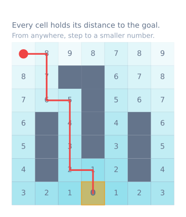
Flood fill assigns every cell a number: its distance to the goal. The goal cells get zero. From there, each neighboring cell that is not blocked gets one more than its lowest neighbor, spreading outward until every reachable cell has a value.
The robot never stores a route. It just stands in a cell, looks at its neighbors, and steps to any one whose number is exactly one lower. The distance field is the plan, which is why it recovers gracefully when the map changes.
Optimism about unknown walls
The robot cannot see the whole maze, so flood fill treats every wall it has not yet sensed as open. That optimism produces the shortest possible estimate and keeps the robot moving toward the goal instead of exploring aimlessly.
When a sensor reveals a wall that was assumed open, the robot records it—on both sides of the shared edge—and recomputes the distance field. The plan corrects itself, and the robot continues from wherever it is.
Why the first run is not the shortest path
A common surprise: flood fill does not guarantee the shortest route on the first run. Because it acted on optimistic assumptions, it found a way to the goal, not necessarily the best one. Real Micromouse robots use two phases:
- A search run that explores enough of the maze to build an accurate map.
- A speed run along the shortest path that the completed map reveals.
Early on, efficient exploration matters more than first-run optimality.
Flood fill versus BFS and A*
Breadth-first search and A* plan over a graph you already know. Flood fill is designed for a maze you are still discovering: it re-floods whenever a new wall appears. Mathematically the flood is a breadth-first distance computation—the difference is that flood fill expects the map to keep changing and is cheap to recompute.
It also beats simple wall following (always keep one hand on a wall), which cannot reach a goal in the center of the maze and rarely finds a short route.
The sensing-planning-moving loop
void planOneCell(Maze& map, Robot& robot) {
  map.observe(robot.cell(), robot.senseLeftFrontRight());
  map.floodFill(centerGoals);
  Cell next = map.bestDescendingNeighbor(robot.cell());
  robot.turnAndMoveTo(next);
}
Keep sensing, mapping, planning, and motion as separate steps. That boundary is what lets the same planner run in a browser simulator, on your desktop, and on an ESP32 with real distance sensors and encoders.
The flood, in full
The distance field is a breadth-first expansion from the goal, and it is short enough to write out completely:
const uint8_t N = 16;                       // 16 x 16 maze
uint8_t dist[N][N];                         // distance to goal, per cell
uint8_t walls[N][N];                        // bitmask: 1=N, 2=E, 4=S, 8=W

// A simple ring buffer beats a std::queue on a microcontroller.
uint8_t queueR[N * N], queueC[N * N];

void floodFill(const uint8_t goals[][2], uint8_t goalCount) {
  memset(dist, 255, sizeof(dist));          // 255 = unreachable

  uint16_t head = 0, tail = 0;
  for (uint8_t g = 0; g < goalCount; g++) {
    const uint8_t r = goals[g][0], c = goals[g][1];
    dist[r][c] = 0;
    queueR[tail] = r; queueC[tail] = c; tail++;
  }

  const int8_t dr[4] = {-1, 0, 1, 0};       // N, E, S, W
  const int8_t dc[4] = { 0, 1, 0, -1};

  while (head < tail) {
    const uint8_t r = queueR[head], c = queueC[head];
    head++;

    for (uint8_t d = 0; d < 4; d++) {
      if (walls[r][c] & (1 << d)) continue;             // wall in the way

      const int8_t nr = r + dr[d], nc = c + dc[d];
      if (nr < 0 || nr >= N || nc < 0 || nc >= N) continue;

      if (dist[nr][nc] > dist[r][c] + 1) {              // 255 means unvisited
        dist[nr][nc] = dist[r][c] + 1;
        queueR[tail] = nr; queueC[tail] = nc; tail++;
      }
    }
  }
}
That is the whole algorithm. On a 16×16 maze it visits at most 256 cells and runs in well under a millisecond on an Arduino — which is why re-flooding on every newly discovered wall is entirely affordable, and why nobody bothers with incremental updates.
Recording a wall on both sides
The single most common flood-fill bug is not in the flood at all. A wall is shared between two cells, and recording it on only one side produces a map where the robot can pass through it in one direction and not the other:
void setWall(uint8_t r, uint8_t c, uint8_t dir) {
  walls[r][c] |= (1 << dir);

  const int8_t dr[4] = {-1, 0, 1, 0};
  const int8_t dc[4] = { 0, 1, 0, -1};
  const int8_t nr = r + dr[dir], nc = c + dc[dir];
  if (nr < 0 || nr >= N || nc < 0 || nc >= N) return;

  walls[nr][nc] |= (1 << ((dir + 2) % 4));   // the same wall, from the other side
}
The (dir + 2) % 4 is the opposite direction — north becomes south, east becomes west. The
symptom of getting this wrong is a robot that plans a route straight through a wall it
personally recorded, which is a genuinely confusing thing to watch.
Memory, on an Arduino
A 16×16 maze on an Uno’s 2 KB of SRAM is tight but workable, and the arithmetic is worth doing before you find out the hard way:
| Structure | Size | Notes |
|---|---|---|
dist[16][16] as uint8_t |
256 B | Distances never exceed 255 in a 16×16 maze |
walls[16][16] as uint8_t |
256 B | 4 bits used per cell; packing saves 128 B and costs clarity |
Queue, two uint8_t arrays |
512 B | The worst case is every cell queued once |
| Total | 1024 B | Half the Uno’s SRAM, before anything else |
The queue is the expensive part and the easiest to shrink: a single array of packed r<<4|c
bytes halves it to 256 B. If you are still tight, packing the wall map into 2 bits per cell
recovers another 192 B. Most people reach for an ESP32 or a Mega at this point instead, and
that is a reasonable call — but the exercise of making it fit is itself instructive.
Choosing goal cells
A standard Micromouse goal is a 2×2 block at the centre, not a single cell, and that is not a detail. Seeding all four cells with distance 0 means the robot heads for whichever face of the block it can reach most cheaply — which is both faster and more robust than committing to one specific cell it may have to approach from an awkward direction.
The code above already handles it: pass all four cells in goals, and the flood begins from
every one of them simultaneously. This is a genuine advantage of the distance-field approach —
multiple goals cost nothing, whereas A* would need a modified heuristic.
Exploring properly
Flood fill tells the robot where to go given what it knows. It says nothing about what it should learn, and a robot that only ever descends the gradient will reach the goal without having seen most of the maze — which makes the speed run’s “shortest path” shortest only among the corridors it happened to walk.
| Strategy | Explores | Speed-run quality | Time cost |
|---|---|---|---|
| Descend the gradient only | The minimum | Often well off optimal | Fastest |
| Descend, then return to start by the same rule | A little more | Better | Low |
| Explore until every cell adjacent to the known path is seen | Most | Near-optimal | Moderate |
| Full exhaustive exploration | Everything | Optimal | Slow |
The usual competition compromise is the second or third row: reach the goal, then flood back toward the start and drive that, which naturally reveals a different set of corridors. Two traversals typically produce a map good enough that the speed run is within a few percent of optimal.
Troubleshooting
| Symptom | Likely cause | Fix |
|---|---|---|
| Robot plans through a wall it just found | Wall recorded on one side only | Record both sides — see setWall above |
| Distance field has 255s in reachable places | Queue overflowed, or the flood ran before walls were set | Size the queue for N × N; re-flood after every observation |
| Robot oscillates between two cells | Two neighbours with equal distance and no tie-break | Prefer the current heading on a tie — it also avoids a needless turn |
| Reaches the goal but the speed run is slow | It explored only the corridor it walked | Explore more before committing to a speed run |
| Works in simulation, fails on hardware | Position drift, not the algorithm | The planner is fine; the robot is not in the cell it thinks |
| Runs out of RAM | The queue | Pack cells into a single byte; consider a Mega or ESP32 |
| Distances look right, robot turns the wrong way | Direction bitmask order mismatched between sensing and flooding | One order (N, E, S, W) everywhere, defined once |
That fifth row is the important one, and it is worth stating plainly: the algorithm is not the hard part of a Micromouse. Flood fill is forty lines and you can verify it completely in the simulator with no hardware. The hard part is that after ten cells the robot is no longer where it believes it is, and a perfect plan executed from a fictional position drives into a wall.
Try it yourself
Step through the Maze Solver Simulator one cell at a time and watch the distance field recompute each time the robot discovers a wall. Seeing the numbers change is the fastest way to understand why the robot always has a plan.
Explore the graph
Part of these builds
Projects and learning paths that include this tutorial.
Further reading